 Statistics
How Do You Calculate Variance? A Simple Explanation With Real Examples
How to calculate variance step by step: find the mean, the deviations, the squared deviations and the sum of squares, with a fully worked example.
データ入力
データ値を入力すると結果が表示されます
Variance tells you how spread out a set of numbers is: how far, on average, the values sit from their mean once each distance is squared. This calculator takes a list of numbers and works that out for you. It finds the mean, subtracts it from every value, squares the differences, adds them up and divides, then shows each of those steps so you can follow or check the working.
It is written for students checking homework, teachers preparing examples, and anyone who needs a quick, reliable figure for a report or a spreadsheet. You get both versions of the answer: sample variance (s²), which divides by n − 1 and is the one to use when your numbers are a sample from a larger group, and population variance (σ²), which divides by n and is for when you have every value in the group. The standard deviation, mean, range and sum of squares come with it.
To use it, type or paste your numbers into the box above, separated by commas, spaces or new lines. You can paste a column straight from Excel or Google Sheets. Choose Sample or Population, and the results and chart update as you type. Everything is calculated in your browser, so your data is not uploaded anywhere.
分散計算の背後にある数学的背景を理解しましょう。
インタラクティブ: 数式内の記号の上にマウスを置くかタップすると、その記号が何を表しているかが表示されます。
Uses n − 1 (Bessel's correction) for an unbiased variance estimate from sampled data. This adjustment accounts for degrees of freedom when the true population mean is unknown.
Divides by n directly. No correction needed because the population mean (μ) is the true mean of the whole population.
How Data Flows Through the Formula
母集団の分散と標本分散は、1 か所、 それは約数で異なります。母集団分散は、差の二乗和をn (総数) で割ります。標本分散を n − 1 (ベッセル補正) で除算して、標本データから不偏分散推定値を生成します。この補正はサンプルが小さい場合に最も重要です。データセットが大きい場合、その差は小さくなります。
分散は、データセット内の各数値が平均からどの程度離れているかを測定します。以上が分散計算の手順です。
分散を計算するには、平均からの差の二乗の平均を求めます。このプロセスは母集団分散と標本分散の場合と同じです。唯一の違いは、最後に n で割るか、n − 1 で割るかです。この統計的分散計算は、調査分析から機械学習の特徴選択まで、あらゆるデータセットに対して機能します。
試してみましょう: 数字を入力して各ステップを確認してください
3 ~ 8 個の数字をカンマで区切って入力します。以下の手順では、データの分散をリアルタイムで計算します。
平均値を求める (平均)
データセット内のすべての値を加算し、カウントで割ります。 [4、8、6、5、3] の場合、平均は (4+8+6+5+3) ÷ 5 = 5.2 となります。この平均は、すべての分散計算の中心点になります。
平均を減算して偏差を取得する
各数値から平均を減算して偏差を求めます。負の偏差は、値が平均を下回っていることを意味します。正の値が上です。偏差の合計は常に 0 に等しくなります。
各偏差を二乗する
各偏差を二乗して正にします。これにより、平均値を下回る偏差と平均を上回る偏差が互いに打ち消し合わなくなることが保証されます。二乗法では、外れ値の重みも大きくなります。
偏差の二乗を合計する
すべての二乗偏差を合計します。この合計は二乗和 (SS) と呼ばれます。私たちのデータでは、1.44 + 7.84 + 0.64 + 0.04 + 4.84 = 14.8 となります。
分散を求める除算
二乗和を N (母集団の場合) または n − 1 (サンプルの場合) で割ります。標本分散の場合、14.8 を 4 で割ると 3.7 が得られます。母集団分散の場合、5 で割ると 2.96 になります。
サンプル データセットの分散を計算してみましょう: 4、8、6、5、3、7、2、9。
Consider the data set: 4, 8, 6, 5, 3, 7, 2, 9. We'll calculate both sample variance (s²) and population variance (σ²) for these 8 values. Watch the bar chart below — it shows each data point, the mean line, and the squared deviations as you scroll through each step.
The mean is the center of the data set — every deviation is measured from this point. In the bar chart above, the dashed line marks x̄ = 5.5.
| xᵢ | 偏差 (x − x̄) | 二乗偏差 (x − x̄)² |
|---|---|---|
| 4 | −1.5 | 2.25 |
| 8 | 2.5 | 6.25 |
| 6 | 0.5 | 0.25 |
| 5 | −0.5 | 0.25 |
| 3 | −2.5 | 6.25 |
| 7 | 1.5 | 2.25 |
| 2 | −3.5 | 12.25 |
| 9 | 3.5 | 12.25 |
Each row shows one data point, its deviation from the mean, and the squared deviation. Notice how values far from x̄ (like 2 and 9) produce much larger squared differences.
This sum of squares (42) represents the total squared distance of all data points from the mean. It's the numerator in both variance formulas.
計算機を使用せずに手動で分散を計算するには、次のチェックリストの手順に従ってください。
すべての数字を明確にリストします。値の数 (n) を数えます。
すべての数値を加算し、n で割ります。この値に注目してください。
各生の値から平均を引きます。否定的な人もいるだろう。
それぞれの差を掛け合わせます。すべての値は正でなければなりません。
差の二乗を合計します。これが平方和です。
この最後のステップで分散が得られます。
データセットにグループのすべてのメンバーが含まれている場合は、母集団の分散を使用します。つまり、n − 1 ではなく n で割ります。
母集団分散は、データセットに標本ではなく母集団全体からのすべての観測値が含まれている場合に適用されます。例: 会社の全従業員、クラス内のすべてのテストのスコア、品質管理中のバッチ内のすべての製品。この式では、μ (母集団の真の平均) を使用し、n (全数) で割ります。ベッセルの訂正はありません。自由度調整はありません。
インタラクティブ: サンプルサイズが分散に与える影響
スライダーをドラッグして、σ² と s² の差が母集団サイズに応じてどのように変化するかを確認します。 n が小さい場合、ギャップは大きくなります。 n が大きくなるにつれて、標本分散は母集団分散に向かって収束します。
Convergence: s² approaches σ² as n grows
9 個の特殊な統計計算機 - それぞれにパーソナライズされたステップバイステップのソリューション、公式、FAQ が含まれています。問題に合ったツールを選択してください。
標準偏差 電卓
ステップバイステップのソリューションで標準偏差を瞬時に計算します。データセットを入力して、母集団 SD (σ)、サンプル SD (s)、分散、平均などを取得します。無料、高速、正確。…
平均 電卓
あらゆるデータセットの平均値を瞬時に計算します。分散、標準偏差、中央値などとともに算術平均を取得します。無料の段階的なソリューション。…
サンプルの分散 電卓
ステップバイステップのソリューションでサンプル分散 (s²) を即座に計算します。不偏推定にはベッセル補正 (n−1) を使用します。標準偏差、平均などを取得します。無料かつ正確。…
母集団の分散 電卓
ステップバイステップのソリューションで母集団分散 (σ²) を瞬時に計算します。母集団全体がある場合、正確な分散を求めるには N で割ります。無料のオンライン母集団分散計算ツール。…
変動係数 電卓
変動係数 (CV) を瞬時に計算します。単位やスケールが異なるデータセット間の相対的な変動を比較します。分散と標準偏差を使用した無料のステップバイステップのソリューション。…
パーセンテージの差異 電卓
値間の分散のパーセンテージを計算するか、分散を平均のパーセンテージとして表します。変動係数、分散、標準偏差、および段階的なソリューションを取得します。無料ツール。…
プールされた分散 電卓
複数のグループまたはサンプルからプールされた分散を計算します。 2 標本 t 検定、ANOVA、およびメタ分析の標本分散を組み合わせます。段階的なソリューションを備えた無料のオンラインプール分散計算ツール。…
ポーカーの分散 電卓
ポーカーの分散を計算し、任意の数のハンドで予想される結果を理解します。ポーカーにおける勝率の分散、ダウンスイングの確率、標準偏差を分析します。無料ツール。…
分散について知っておくべきことのすべて。
6, 7, 5, 9, 12, 15の分散は以下のように計算されます。平均 = (6+7+5+9+12+15) / 6 = 9。平均からの偏差の二乗: (6−9)²=9, (7−9)²=4, (5−9)²=16, (9−9)²=0, (12−9)²=9, (15−9)²=36。偏差の二乗和 = 74。母集団分散 (σ²) = 74 / 6 ≈ 12.33。標本分散 (s²) = 74 / 5 = 14.8。数値全体が全データセットである場合は母集団分散を使用します。
分散、標準偏差、実用的な統計の解説記事とチュートリアルをご覧ください。
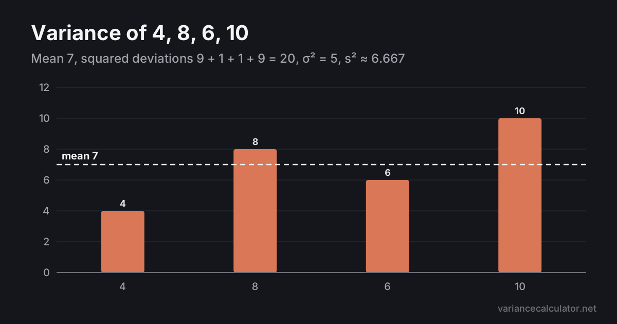
Statistics How to calculate variance step by step: find the mean, the deviations, the squared deviations and the sum of squares, with a fully worked example.
 Statistics
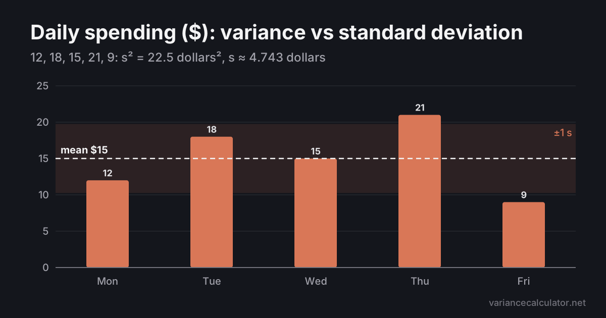
Variance and standard deviation describe the same spread on different scales. How they connect, what their units mean, which to report, and a worked example.
 Statistics
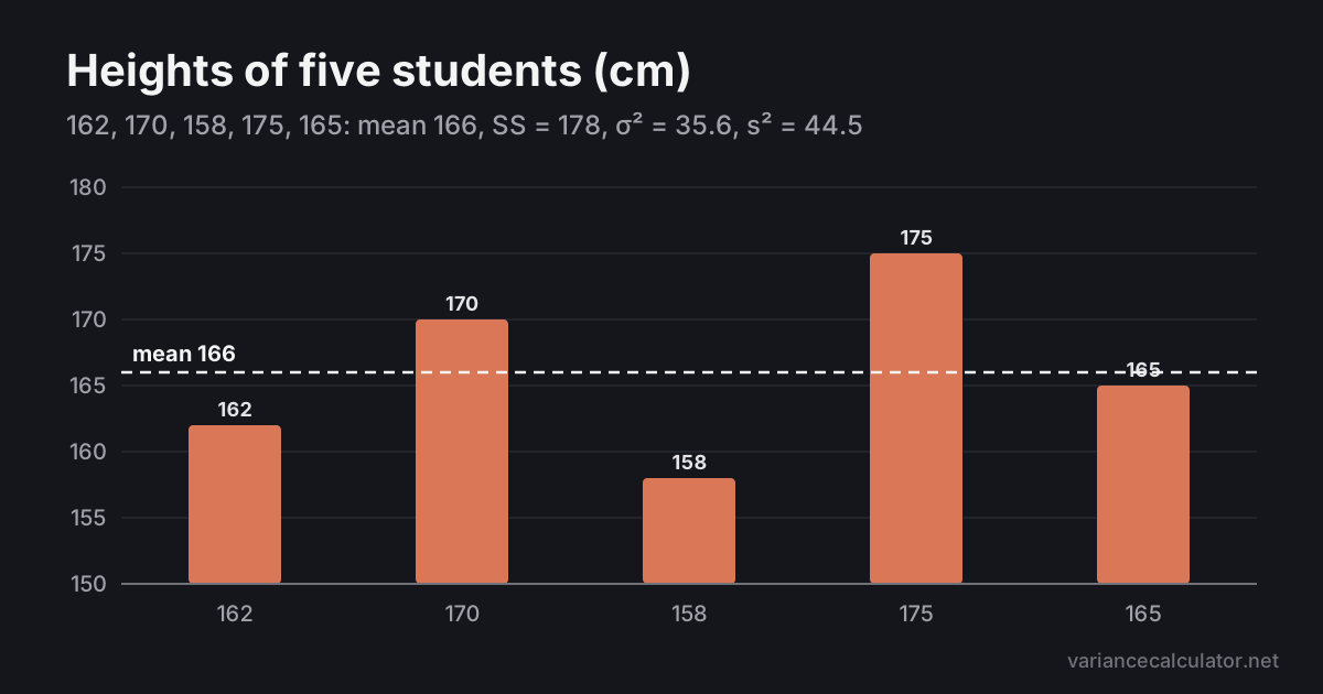
When to use sample variance and when to use population variance, why dividing by n − 1 corrects a bias, and a worked example with both formulas.